Querying a schedule with SQL

Prebuilt views answer the common questions well. But schedule work has a long tail of uncommon ones — the ad-hoc “how many, of what, where, filtered by this odd condition” that no dashboard anticipated. For those, the fastest tool is often the oldest one: write the query yourself.

This post is about treating a parsed SSIM schedule as a set of tables you can ask read-only SQL against — to verify a number behind a chart, answer a one-off question, or export exactly the slice you need — all locally, with the schedule never leaving your machine.

From a fixed-width file to tables

A raw SSIM file is not something you can query. It’s fixed-width, positional text: meaning lives at byte offsets, a leg is a pattern over a period, times are local with a mode and offset. SQL wants the opposite — typed columns, one clean value per field. The bridge is parsing: read the file faithfully, type every field, and present the result as ordinary relations.

Once that’s done, a schedule looks like a small, familiar set of tables:

• flights — one row per flight leg: carrier, flight number, board and off points, operating days, times, equipment, derived seat capacity.
• segments — the segment-level detail (the Type 4 data elements) attached to their parent leg.
• carriers — the airline records: designator, season validity, time mode.
• pre-aggregated relations — ready-made rollups (routes, calendar day-counts, and the like) so the heavy folds are already done.

From there it’s just SQL.

A small example

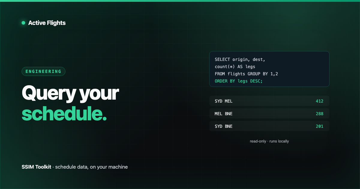
Say a capacity chart shows weekly departures per market and a number looks off. Rather than trust or distrust the chart, check it directly:

(Illustrative. A real query would normalize the count to a typical week using the operating-days expansion rather than a raw count(*).) Now the chart’s number has a provenance you can see. That’s the whole appeal of dropping to SQL: no black box between the question and the rows.

Read-only on purpose

The queries you run against a schedule are strictly for reading. There is no reason to INSERT, UPDATE, DELETE, or reshape the underlying store from an analysis query — and every reason not to. The parsed schedule is a faithful, trailer-verified representation of the source file; an analyst’s ad-hoc query should never be able to mutate it.

So read-only is treated as a security property, not a convention. The query surface accepts a single read statement and refuses anything that would write, alter, attach, or reach outside the schedule. You get the full expressiveness of SQL for asking questions, and none of the ways it could damage the thing you’re asking about.

A schedule query answers questions about the data. It should never be able to change the data. Enforce that at the surface, not in a code review.

Local, and private

The other half is where this runs. Schedule data is commercial, and often confidential. The moment answering “how many weekly departures on this market” means uploading the file to someone else’s service, you’ve made a small analytical convenience into a data-governance decision.

The local-first answer is to run the query against a local serving store on your own machine. The schedule stays where it is; the SQL executes beside it; the result is yours. Nothing about your network — the markets you serve, the carriers you’re studying — travels anywhere to answer a question about it.

SQL or a warehouse? Both are right

Dropping to local SQL isn’t the opposite of pushing schedules to a warehouse — they answer different needs.

Local read-only SQL	Warehouse / lakehouse
One schedule, one machine, right now	Many schedules, shared, over time
Verify a number, answer an ad-hoc question	Company-wide joins with other datasets
Nothing leaves your machine	A modelled, governed shared asset
No pipeline to stand up	Worth the pipeline at scale

The exploratory question you have today wants local SQL. The cross-dataset analysis your whole team runs repeatedly wants the warehouse. A good workflow uses local SQL to figure out the query, then exports — CSV, JSON, or Parquet — into the warehouse when it’s worth keeping.

Letting an assistant drive it — read-only

There’s a newer way to ask these questions: let an AI assistant write the SQL for you. The pattern here keeps the determinism on the inside. Your own AI assistant connects to a built-in, read-only, on-device MCP server and can query the schedule through the same read-only surface — it asks, the deterministic engine answers. The assistant never computes the numbers itself and never gets a way to write; it’s a natural-language front end to the exact same guarded, local SQL. AI on the outside, determinism on the inside.

Where it fits

The SQL Notebook in SSIM Toolkit is exactly this surface: the parsed schedule exposed as read-only tables — flights, segments, carriers, and the pre-aggregated relations — that you query with SQL and export the result to CSV, JSON, or Parquet. It runs locally against a local serving store, is read-only by construction, and is reachable both by hand and, through the on-device MCP server, by your own AI assistant.

When the prebuilt views don’t have your question, you write it — and the schedule answers, on your machine. More on the SSIM Toolkit product page.